The Basic Deterministic Inventory Models
Before examining the solution of specific inventory models, we provide the notations used in the development of these models.
Q = Number of units ordered per order.
D = Rate of demand.
N = Number of orders placed per year.
TC = Total inventory cost
Co = Cost of ordering per order
C = Purchase or manufacturing price per unit
Ch = Cost of holding stock per unit per period of time.
Cs = Shortage cost per unit.
R = Reorder point
L = Lead time (weeks or months)
t = The elapsed time between placement of two successive orders.
Model I - Economic Order Quantity Model With Uniform Demand
The main problem while purchasing material is how much to buy at a time. If large quantities are bought, the cost of carrying the inventory would be high. To the contrary, if frequent purchases are made in small quantities, costs relating to ordering will be high. So the problem is of indecision. How this problem can be resolved ?
Economic Order Quantity (EOQ) is that size of the order for which the cost of maintaining inventories is minimum. Therefore, the quantity to be ordered at a given time should be determined by taking into account two factors, i.e., the acquisition cost and the cost of possessing materials. We illustrate this model after making the following assumptions:
Assumptions
- Demand rate is uniform over time and is known with certainty.
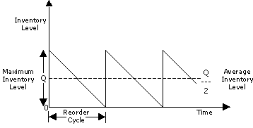
- The inventory is replenished as soon as the level of the inventory reaches to zero. Thus shortages are not allowed.
- Lead time is zero.
- The rate of inventory replenishment is instantaneous.
- Quantity discounts are not allowed.
The inventory costs are determined as follows:
1. Ordering cost = Number of orders per year X Ordering cost per order
= N X Co
= Total annual demand/Number of units ordered X Co
| = | D ---- Q |
X | Co |
2. Carrying cost = Average inventory X carrying cost per unit
| = | Q ---- 2 |
X | Ch |
The total inventory cost is the sum of ordering cost and carrying cost.
| TC = | D ---- Q |
Co | + | Q ---- 2 |
Ch |
The total cost is minimum at a point where ordering cost equals carrying
cost. Thus, economic order quantity occurs at a point where
Ordering cost = Carrying cost
| D ---- Q |
Co | = | Q ---- 2 |
Ch |
Thus, optimal Q* (EOQ) is derived to be
| EOQ = | Q* = | 2DCo ------------ Ch |
|||
| The period t is given by t* = | Q* |
= | 2Co ---------- ChD |
||
| Optimal number of orders per year is given by N* = | D ---- Q* |
= | 1 ----- t* |
||
| Minimum total yearly inventory cost TC* = |
|
2DCoCh | |||
 Example 1
| Annual usage | 500 pieces |
|---|---|
| Cost per piece | Rs. 100 |
| Ordering cost | Rs. 10 per order |
| Inventory holding cost | 20% of Average Inventory |
Solution.
D = 500 pieces
Co = 10
Ch = 100 X 20% = Rs. 20
| EOQ = | (2 X 10 X 500) ---------------- 20 |
EOQ = 22 pieces (rounded)
Example 2
The Newtech Hardware Company sells hardware items. Consider the following information.
Annual sales = Rs. 10000
Ordering cost = Rs. 25 per order
Carrying cost = 12.5% of average inventory value.
Find the optimal order size, number of orders per year, and cycle period.
Solution.
D = Rs. 10000, Co = Rs. 25, Ch = 12.5% of average inventory value/unit
| EOQ = | Q* = | (2 X 25 X 10000) ---------------- (0.125 ) |
= | Rs. 2000 | ||
| t* = | Q* |
= | 2000 -------- 10000 |
= | 1/5 yrs = 73 days | |
| N* = | 1 ---- t* |
= | 1 ----- 1/5 |
= | 5 | |


